
|
Home
| pfodApps/pfodDevices
| WebStringTemplates
| Java/J2EE
| Unix
| Torches
| Superannuation
|
| About
Us
|
|
|
Arduino Date and Time using millis() and pfodApp™
|
by Matthew Ford 26th April 2018 (original
21st April 2018)
© Forward Computing and Control
Pty. Ltd. NSW Australia
All rights reserved.


This tutorial shows you how to use your Arduino
millis()
timestamps to plot data against date and time on your Android mobile
using pfodApp.
No
Arduino or Android programming required.
pfodApp also logs sufficient data so that you can later reproduce the
date/time plots in a spreadsheet.
NO RTC or GPS module is needed, however if your Arduino project has an RTC (Real Time Clock) or a GPS module they can also be used. In those cases the pfodApp plots will automagically correct for timezone, RTC drift and GPS missing leap seconds. No special Arduino code is required for these corrections. As always with pfodApp, the data received is logged exactly as is, un-corrected, however the log file also contains sufficient information to allow you to apply these corrections yourself when you download the logs to your computer. See below for examples of this post-processing.
A wide variety of time and date X-axis formatting is supported, all of which are completely controlled by short text strings in your Arduino sketch. No Android programming is required.
pfodApp will connect via WiFi, Bluetooth Classic, BLE and SMS. The free pfodDesigner generates complete Arduino sketches for date/time plotting/logging to connect to wide variety of boards. No Arduino programming is required.
This tutorial will use an Adafruit Feather52 as the example Arduino board, which connects via BLE.
This tutorial covers three cases:-
1) Your
microprocessor project only has millisecond timestamps –
millis()
2) Your microprocessor project has a Real Time Clock
(RTC) – pfodApp automatically corrects for drift.
3) Your
microprocessor project has a GPS module – pfodApp automatically
corrects for leap second (18 secs as at 2018).
There are two parts to using milliseconds for date and time. One is for plotting the data against either elapsed time or date/time and the other part is re-creating the date and time from the the logged rawdata millisecond timestamps. pfodApp does not modify the raw data received from the pfodDevice (the Arduino micro). It just logs exactly the bytes received.
First use the free pfodDesigner to generate an Arduino sketch for your micro that will send the milliseconds and data measurements to pfodApp for plotting/logging. This example creates a menu for the Adafruit Feather 52 BLE board that reads A0. The tutorial on Adafruit Feather nRF52 LE - Custom Controls with pfodApp goes through the pfodDesigner steps to create a menu for the Feather nRF52 that includes a Chart button, so check it out for more details. In this tutorial we will add just a chart button and use the new X-axis format options to plot the A0 readings against elapsed time and date/time.
The first part of this tutorial will go through using the free pfodDesigner to create a sample date/time chart on your Android mobile. When you are satisfied with the display you can generate the Arduino sketch that will reproduce that when you connect with pfodApp. No Android Programming is required and since pfodDesigner generates complete Arduino sketches for a wide variety of Arduino boards, no Arduino programming is required either.
Download the free pfodDesigner app from Google Play, open it and click on “Start new Menu”

Click on the “Target Serial” and then on the “Bluetooth Low Energy” button to display the list of some 11 BLE boards (scroll down to see the other choices). Select on Adafruit Bluefruit Feather52.

Go back to the Editing menu and click on “Edit Prompt” and set a suitable prompt for this menu, e.g. “Feather52” and text bold and size +7. The background colour was left as the 'default' White

Go back and click on “Add Menu Item”, scroll down and select “Chart Button” which opens the chart button edit screen. You can make any change to the button's appearance here. In this case button's text was change to “Date/Time plot of A0” and the other defaults were left as is.

Click on the “Date/Time plot of A0” button to open Editing Plots screen, where you can access the chart label, X-axis format, plot data interval and (by scrolling down) the plot settings themselves. Edit the Chart Label to something suitable, e.g. “A0 Volts”.

Scroll down and for Plots 2 and 3 open Edit Plot and click Hide Plot to remove them from the chart display.

Then click on “Edit Plot 1” and set a plot label (e.g. A0), yAxis units (e.g. Volts), display max of 3.6V and connect to I/O pin A0.

Scroll back up and click on “Chart Preview” to most recent 0 sample data points, at 1sec intervals, plotted against elapsed time in mins:secs.

For all elapsed time plots leading zero units are not displayed so in this plot only those time > 1min have leading minutes shown.
For elapsed time plots the leading unit just keeps increasing as the time goes on. To see an example of this go back to the “Editing Plots” screen and increase the Plot Data interval to 15mins (bottom of this screen)

Then click on Chart Preview to show the same sample data but now with 15min intervals between samples. As you can see the minutes part of mm:ss just keeps increasing.

Now go back and click on the X-axis button to show a small selection of all the possible X-axis data/time formats (scroll down for more)

Here is a selection of chart previews using different X-axis formats.
The date/time plots shown here are in the 'local' timezone. There are also format options to plot date/time in UTC. For a complete set of possible date/time format options see the pfodSpecification.pdf.
Once you are happy with your chart's format and data interval, you can to the “Editing Menu_1” screen and scroll down and “Generate Code” for you chosen target board. Here is the a sample sketch for the Adafruit Feather52 using 1sec data intervals and a mm:ss elapsed time format, pfodFeather52_timeplot.ino
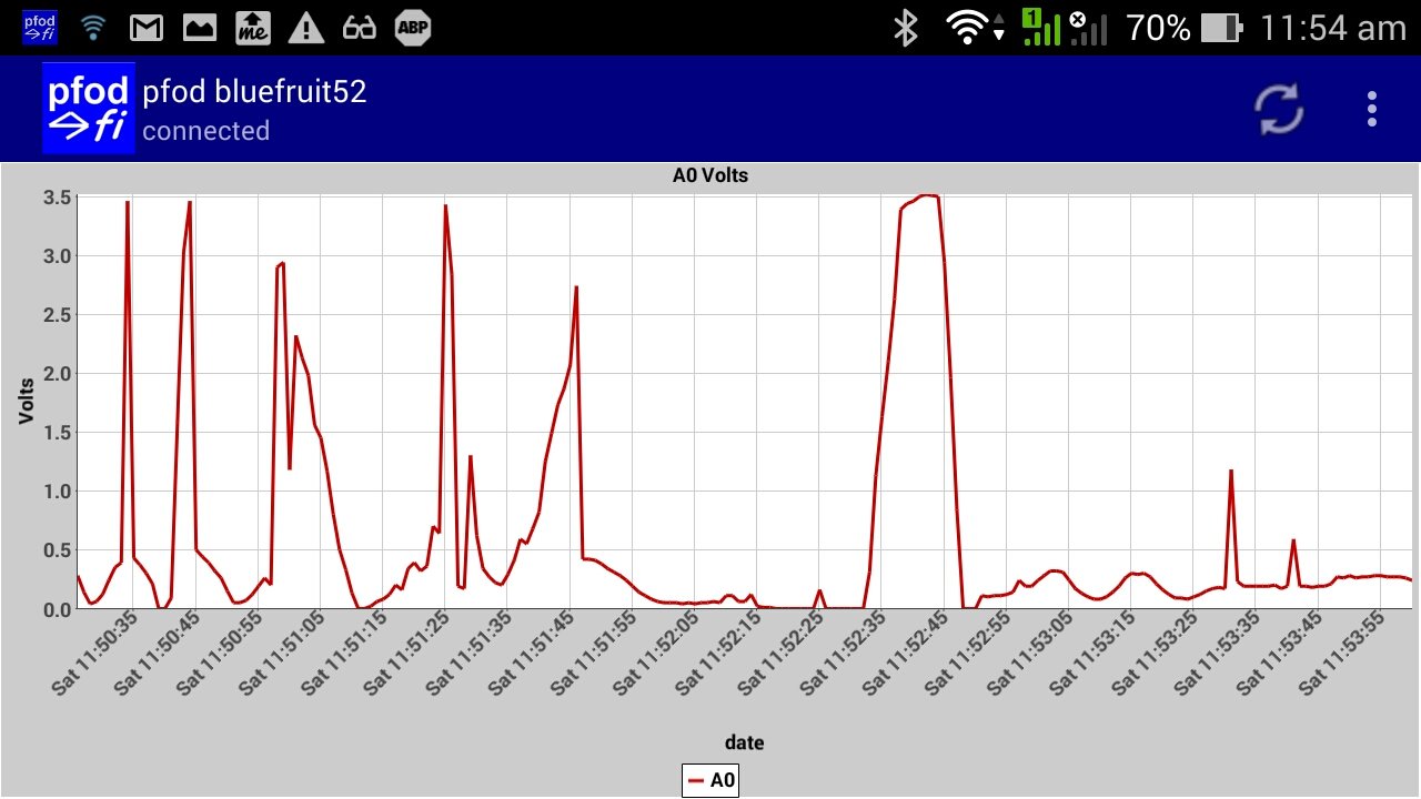
Here is a plot of A0 from the Feather52

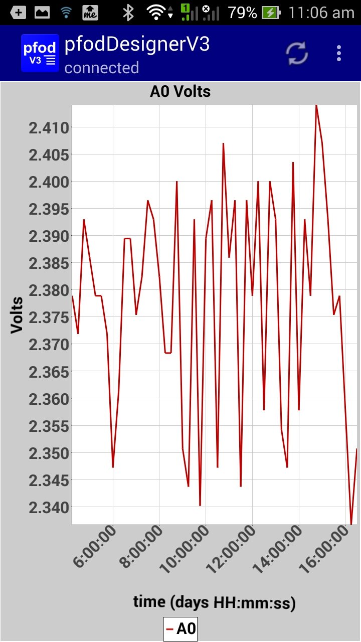
Changing the format to Weekday hr:mins:sec (~E HH:mm:ss) and re-generating the code (pfodFeather52_dateplot.ino) gives a plot like
You can edit the X-axis format directly in your Arduino sketch, as described next.
When pfodApp connects, it remembers its 'local' and UTC time and requests the pfodDevice's (the Arduino board's) current plot data timestamps. Using this information pfodApp can then plot millisecond timestamps as either elapsed time i.e. converting milliseconds to hrs mins sec etc, or plot the date and time the millisecond timestamps represent relative to when the connection was made and the pfodDevice's current time was requested.
Looking in the Arduino generated sketch (e.g. pfodFeather52_dateplot.ino), there are three small bits of code that handle the Arduino side of the plots.
The loop() code section that handles the pfodApp's {@} current time request
      // handle {@} request
    } else if('@'==cmd) { // pfodApp requested 'current' time
      plot_mSOffset = millis(); // capture current millis as offset rawdata timestamps
      parser.print(F("{@`0}")); // return `0 as 'current' raw data milliseconds
You could just return the current value of millis(), but
millis() wraps around back to 0 every 49.7 days, which would
make the plot jump backwards. So instead the code remembers the
current millis() value when the {@} request was made,
and returns {@`0} i.e. a current millisecond timestamp of
zero. Then when sending the rawdata points the sketch uses
    plot_1_var = analogRead(A0); // read input to plot
    // plot_2_var plot Hidden so no data assigned here
    // plot_3_var plot Hidden so no data assigned here
    // send plot data in CSV format
    parser.print(millis()-plot_mSOffset);// time in milliseconds
    ….
so that the millisecond timestamp sent with the data starts at 0 and increases up to 49.7days. If you stay connected continually for 49.7days then you will see the plot jump backwards by ~50days. Disconnecting and re-connecting once each 49.7 days avoids this.
The third part of the date/time plot is the plot message.
    } else if('A'==cmd) { // user pressed -- 'Date/Time plot of A0'
      // in the main Menu of Menu_1
      // return plotting msg.
      parser.print(F("{=A0 Volts~E HH:mm:ss|date|A0~~~Volts||}"));
When
the user presses the “Date/Time plot of A0” button,
pfodApp sends the {A}
cmd
to the pfodDevice and the pfodDevice responds with the plot message,
{=...
{=A0
Volts~E HH:mm:ss|date|A0~~~Volts||}
which
contains the X-axis format E
HH:mm:ss Java
SimpleDateFormat formats are acceptable here. pfodApp
Data Logging and Plotting and the pfodSpecification.pdf
have more details on the plot message.
By default, pfodApp logs all the incoming rawdata to a log file on your mobile, unless you have disabled this logging in the connection edit screen, see the pfodAppForAndroidGettingStarted.pdf
When you edit pfodApp, a brief message displays with the location and name of the log file, e.g. /pfodAppRawData/pfod_bluefruit52.txt That file is in CSV format, comma delimited, and after transferring it to your computer (see the pfodAppForAndroidGettingStarted.pdf for transfer options), you can open it in a spreadsheet to plot the data.
Here is first few lines of a the log file.
// pfodApp V3.0.360,local time,UTC,mS per day,pfod bluefruit52 current time(mS),pfod bluefruit52 current time,
// connected at,2019/04/20 11:32:50.238,2019/04/20 01:32:50.238,86400000,0,
366,0.25,,
1366,0.29,,
2366,0.31,,
3366,0.33,,
4366,0.33,,

Above you can see the 'local' and UTC time that pfodApp connected to the Feather52 and the current time in mS that the Feather52 reported via the {@..} response. The last column is blank, because there is no RTC or GPS and so no current time in yyyy/MM/dd time was reported by the Feather52.
To plot the data against elapsed time, subtract the current time (mS) from the millisecond time stamp and then divide by the mS per day value. Here is the spreadsheet with the formula added and the result plotted. The spreadsheet, below, (pfod_bluefruit52.xls) is an OpenOffice spreadsheet saved in Excel format.

In
OpenOffice, the plot is a scatter plot and the x-axis of the plot was
formatted in HH:MM:SS
Note:
the spreadsheet date/time formats are NOT the same as the plot
formats used by pfodApp. For
example in pfodApp, MM is months and mm is minutes.
To
plot against date and time, you only need to add the connection time
to the spreadsheet time and replot. (pfod_bluefruit52_date.xls)
Note:
The local time and UTC were imported as text in my spreadsheet so I
needed to remove the leading ' before using them in a formula.

As mentioned above in How does pfodApp plot
Date/Time from millis()?, if
you remain connected continuously for more then 49.7 days the
millisecond timestamps will wrap around back to zero. A few lines of
code can avoid this but it is not recommended.
First how to avoid the wrap around. Add another unsigned int variable to keep track of the number of times the timestamps wrap around and print the combined result in HEX.
uint_t mSwrapCount = 0;
uint32_t lastTimeStamp = 0;
    …
    plot_1_var = analogRead(A0); // read input to plot
    // plot_2_var plot Hidden so no data assigned here
    // plot_3_var plot Hidden so no data assigned here
    // send plot data in CSV format
    uint32_t timeStamp =  millis()-plot_mSOffset;
    if (timeStamp < lastTimeStamp) {
      // timeStamp wrapped back to 0
      mSwrapCount++;  // add one to count
    }
    lastTimeStamp = timeStamp;
    parser.print("0x"); parser.print(msWrapCount,HEX); parser.print(timeStamp,HEX);// time in milliseconds in HEX
    ….
When returning the {@.. response clear the mSwrapCount as well.
      // handle {@} request
    } else if('@'==cmd) { // pfodApp requested 'current' time
      plot_mSOffset = millis(); // capture current millis as offset rawdata timestamps
      mSwrapCount = 0; // clear wrap count.
      parser.print(F("{@`0}")); // return `0 as 'current' raw data milliseconds
The timestamps will now give the 'correct' value for the next 40.7days * 65536 ~= 7308 years.
pfodApp will automatically convert the hex timestamps
for plotting and log them exactly as received, i.e. in hex. In the
spreadsheet you use this formula to convert the hex string, in A2, to
mS (where A1 is any empty cell)
=HEX2DEC(REPLACE(A2;1;2;A1 ))
As shown above, it is easy to extend the mS timestamps to longer than 50 days. However you probably don't want to do that because they become increasingly in-accurate. A typical 16Mhz crystal used to create the millis() results in the micro has an accuracy of ~50ppm (parts per million). This means that after 49.7 days the millisecond timestamp can be out by 3 ½ mins and that ignores the effect of temperature on the crystal accuracy.
Over short connection periods, this in-accuracy is not a problem as the {@.. response re-synchronizes the millisecond timestamp to the mobile's date/time on each re-connection. However if you want to stay connected for long periods of time (days) and continuously log the data, then you should use something more accurate than the built-in millis(), such as an RTC or GPS module.
There are a number of RTC modules available, one of the more accurate ones is DS3231 e.g. Adafruit's DS3231 module. The stated accuracy is +/-2ppm over 0 to 40C. i.e. ~+/-5 sec/month.
If
you want to plot data that has date/time timestamps, e.g. 2019/04/19
20:4:34, then you need to modify the {@ response to return the
current date/time, e.g. {@`0~2019/4/19
3:33:5}.
Here is some sample code changes to apply to the pfodDesigner
generated sketch for using an RTC module, assuming you are using the
RTClib
library and have added the code initialize the RTC module.
      // handle {@} request
    } else if('@'==cmd) { // pfodApp requested 'current' time
      plot_mSOffset = millis(); // capture current millis as offset rawdata timestamps
      parser.print(F("{@`0"}); // return `0 as 'current' raw data milliseconds
      parser.print('~'); // start string of date/time
      DateTime now = rtc.now()
      sendDateTime(&now); // send yyyy/M/d/ H:m:s to parser.print, pass address & as arg.
      parser.print('}'); // end of {@ response  e.g. {@`0~2019/4/19 3:33:5}
….
// send date time to parser print
void sendDateTime(DateTime* dt) {
  parser.print(dt->year(), DEC);   parser.print('/');
  parser.print(dt->month(), DEC);  parser.print('/');
  parser.print(dt->day(), DEC);    parser.print(' ');
  parser.print(dt->hour(), DEC);   parser.print(':');
  parser.print(dt->minute(), DEC); parser.print(':');
  parser.print(dt->second(), DEC);
}

void sendData() {
  if (plotDataTimer.isFinished()) {
    plotDataTimer.repeat(); // restart plot data timer, without drift
    // assign values to plot variables from your loop variables or read ADC inputs
    plot_1_var = analogRead(A0); // read input to plot
    // plot_2_var plot Hidden so no data assigned here
    // plot_3_var plot Hidden so no data assigned here
    // send plot data in CSV format
    DateTime now = rtc.now();
    sendDateTime(&now); // send yyyy/M/d/ H:m:s to parser.print, pass address & as arg.
    parser.print(','); parser.print(((float)(plot_1_var - plot_1_varMin)) * plot_1_scaling + plot_1_varDisplayMin);
    parser.print(','); // Plot 2 is hidden. No data sent.
    parser.print(','); // Plot 3 is hidden. No data sent.
    parser.println(); // end of CSV data record
  }
}
The ~2019/4/19 3:33:5 part of the {@ response lets pfodApp know what the pfodDevice thinks is the current date and time. Your sketch can then send data with yMd Hms timestamps and pfodApp will plot them either as elapsed time from the connection time OR as date and time, depending on the X-axis format you specify.
When plotting against date and time, the pfodApp plot routine corrects for any 'drift' in the RTC by comparing the pfodDevice's reported current time against the mobile's current time. This correction also handles the RTC being set to a different timezone from the your mobile's local timezone. millis() timestamps continue to work as in Using Arduino millisecond timestamps, above.
Here is an example spreadsheet of room temperatures over an 8 day period, Office_Temp.xls When the log file was imported the first column was marked as YMD to convert the text to a date/time. You still need to remove the leading ' form the local time, UTC and Office Temp current time entries to have the spreadsheet interpret them as dates and times.
To get the same plot that pfodApp shows, you need to calculate the “Corrected Date/Time”. In this case the RTC time is 2 sec behind the mobile's local time, so to each RTC timestamp is added (local time – Office Temp current time) to get the true local time.

For elapsed time plots, create a new column containing the (date/time timstamp – the Office Time current time) and use that as the X-axis in the chart (Office_TempElapsed.xls)

Actually in this case, pfodApp produces nicer elapsed time charts in days hr:mins:sec.
Using a GPS module is similar to using an RTC module, except that GPS modules have milliseconds available, years start at 2000 and the time is missing the UTC leap seconds (see https://tycho.usno.navy.mil/leapsec.html) The GPS date and time is currently 18 secs ahead of UTC, as at January 2018.
The Adafruit GPS library for the Adafruit Ultimate GPS , unlike the RTClib, does not add the 2000 year offset to the GPS years, so that needs to be added when you send the date and time timestamp. Also although the GPS library supplies milliseconds which have very good long term accuracy, they are not very precise. The GPS time updates are only once each 100mS and then there is an extra delay receiving the serial data at a slow 9600 baud and another delay in parsing it. All of which add to the millisecond in-precision when timestamping data readings.
Here are some sample code changes to apply to the pfodDesigner generated sketch for using a GPS module, assuming you are using Adafruit's GPS library and have added the code to receive and parse the messages into a GPS object.
      // handle {@} request
    } else if('@'==cmd) { // pfodApp requested 'current' time
      plot_mSOffset = millis(); // capture current millis as offset rawdata timestamps
      parser.print(F("{@`0"}); // return `0 as 'current' raw data milliseconds
      parser.print('~'); // start string of date/time
      sendDateTime(&GPS); // send yyyy/M/d/ H:m:s to parser.print, pass address & as arg.
      parser.print('}'); // end of {@ response  e.g. {@`0~2019/4/19 3:33:5}
….
// send date time to parser print
void sendDateTime(Adafruit_GPS* gps) {
  parser.print(F("20");  // 20.. year
  parser.print(gps->year, DEC);   parser.print('/');
  parser.print(gps->month, DEC);  parser.print('/');
  parser.print(gps->day, DEC);    parser.print(' ');
  parser.print(gps->hour, DEC);   parser.print(':');
  parser.print(gps->minute, DEC); parser.print(':');
  parser.print(gps->second, DEC);
  // parser.print('.'); if sending milliseconds
  // if you want to send mS you need to pad the gps->milliseconds value with leading zeros
  // i.e. 3 needs to be padded to 003
}

void sendData() {
  if (plotDataTimer.isFinished()) {
    plotDataTimer.repeat(); // restart plot data timer, without drift
    // assign values to plot variables from your loop variables or read ADC inputs
    plot_1_var = analogRead(A0); // read input to plot
    // plot_2_var plot Hidden so no data assigned here
    // plot_3_var plot Hidden so no data assigned here
    // send plot data in CSV format
    sendDateTime(&GPS); // send yyyy/M/d/ H:m:s to parser.print, pass address & as arg.
    parser.print(','); parser.print(((float)(plot_1_var - plot_1_varMin)) * plot_1_scaling + plot_1_varDisplayMin);
    parser.print(','); // Plot 2 is hidden. No data sent.
    parser.print(','); // Plot 3 is hidden. No data sent.
    parser.println(); // end of CSV data record
  }
}
When
plotting against date and time, the pfodApp automatically corrects
for leap seconds. As at Jan 2018, GPS time is 18 sec ahead of UTC.
pfodApp corrects for this by comparing the date/time returned by the
GPS on connection, via the {@
response,
against the mobile's UTC date and time. Creating plots in a
spreadsheet from the pfodApp log file is the same as for RTC modules,
above. Adding the (local time – Office Temp
current time) to the GPS timestamps corrects for the leap seconds.
millis() timestamps continue to work as in Using Arduino millisecond timestamps, above.
Using pfodApp on you Android mobile lets you plot data against date and time or elapsed time, using only Arduino's millis() function. Using the pfodApp log file you can re-produce these date/time plots in a spreadsheet. If your Arduino project has an RTC module, you can log and plot date and the RTC time timestamps, automatically correcting for the RTC 'drift'. If you Arduino project has a GPS module you can log and plot its highly accurate timestamps and pfodApp will automatically correct the the GPS's missing leap seconds.
In all cases the raw data from your Arduino project is logged exactly as received, uncorrected. However the pfodApp log file includes extra data to allow you to re-produce these corrections in a spreadsheet from the downloaded log file.
No Android coding is required. The plot formats are all specified by small text strings in your Arduino sketch. The free pfodDesigner generates complete Arduino data logging and plotting sketches for a wide variety of Arduino boards connecting via WiFi, Classic Bluetooth, BLE and SMS
AndroidTM is a trademark of Google Inc. For use of the Arduino name see http://arduino.cc/en/Main/FAQ
The General Purpose Android/Arduino Control App.
pfodDevice™ and pfodApp™ are trade marks of Forward Computing and Control Pty. Ltd.

Contact Forward Computing and Control by
©Copyright 1996-2020 Forward Computing and Control Pty. Ltd.
ACN 003 669 994